So What is the Associative Scan?
... the all-prefix-sum operation is a good example of a computation that seems inherently sequential, but for which there is an efficient parallel algorithm.
Prefix Sums and Their Applications, Guy E. Blelloch 1993
Recently, I was wondering if it was possible to compute the discounted sum of rewards used in RL using an associative scan - it turns out, it is!. It led me to dig a little bit what there is behind this operation.
So What is the Associative Scan?
Let's say you want to compute the cumulative sum of an array of elements x_1, x_2, ..., x_N, such that y_i = \sum_{j = 1}^i x_i. A straightforward approach would loop over the elements and compute y_i = y_{i - 1} + x_i. More generally, it is very common to apply a function f such that y_i = f(y_{i - 1}, x_i).
The associative scan (also known as parallel scan or prefix sum) is an efficient way to compute all y_i when the function f is associative, i.e. f(f(a, b), c) = f(a, f(b, c)).
Thanks to associativity, we can move the function f around:
f(f(f(a, b), c), d) = f(f(a, b), f(c, d))
The left side is the sequential execution of the scan, running in O(N). The right side runs in O(log N) because the inner calls can be applied in parallel. The parallel execution is usually visualized with the following circuit:
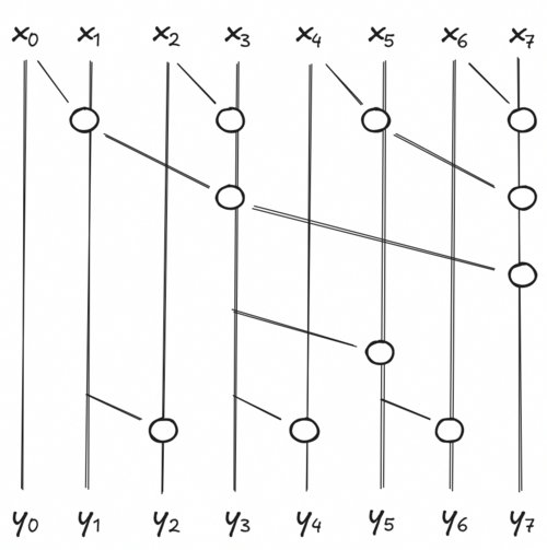
Each circle is an execution of f, and each stage is executed simultaneously. If you look at any y_i and climb up, you will see that every element before x_j are reachable, meaning they took part of the final computation of y_i. Multiple other combinations are possible, but this is one of the most work-efficient. It has a good trade-off between parallelization and computation.
Practical Implementation
At first glance, the image is not easy to reproduce for any vector size. Thankfully, looking at the way JAX implemented it is enough.
Maybe first we can start with a way to compute the sum of an array recursively:
def associative_reduce(fn: Callable[[Array, Array], Array], elems: Array) -> Array:
    if len(elems) < 2:
        return elems

    result = fn(elems[::2], elems[1::2])
    return associative_reduce(fn, result)

elems = jnp.arrange(8)
print(associative_reduce(lambda a, b: a + b, elems))  # [28]
print(jnp.sum(elems))                                 # 28
At every iterations, we separate the array into elements at even and odd
indices. We then apply the function fn in parallel to all
pairs (even, odd) elements. The result contains all partial
sums of our pairs. We can simply call our function again to compute in
parallel the rest of the sum. While this particular implementation is
not very efficient for computing the whole sum (everything could be done
in parallel), you can see how time complexity is reduced from
O(N) to
O(log N). Also, for simplification we
only handle cases where the input is a power of 2.
The associative scan is very similar, but we keep intermediate results and compute missing ones. Let's say at some point of our recursion we have 4 elements (x_0, x_1, x_2, x_3) in our array. If we can compute the exact value of our odds elements y_1 and y_3, it is easy to deduce the value of our remaining even elements y_0 and y_2. y_0 is easy, it is by definition x_0. y_2 is defined recursively by y_2 = f(y_1, x_2).
The last call of our associative scan will compute the last odd element y_{N - 1} and we compute the missing even results of all intermediate calls in order to return the exact value of our elems at every step of our recursion. In general, we compute y_i = f(y_{i - 1}, x_i) for all i even and that is non-zero.
def associative_scan(fn: Callable[[Array, Array], Array], elems: Array) -> Array:
    if len(elems) < 2:
        return elems

    reduced_elems = fn(elems[::2], elems[1::2])
    odd_elems = associative_scan(fn, reduced_elems)
    even_elems = fn(odd_elems[:-1], elems[2::2])
    even_elems = jnp.concat((elems[:1], even_elems))
    return _interleave(even_elems, odd_elems, axis=0)

elems = jnp.arange(8)
print(associative_scan(lambda a, b: a + b), elems)  # [ 0  1  3  6 10 15 21 28]
print(jnp.cumsum(elems))                            # [ 0  1  3  6 10 15 21 28]
Looking at the original figure and this code should make sense, I hope.
Again, this code will only work for arrays that are a power of 2. The
JAX implementation handles inputs of any sizes and even pytrees. Also, I
am cheating a little bit because the _interleave
operation does not exist in the public JAX API, I stole it from
jax._src.lax.control_flow.loops.
Discounted Sum of Rewards
In the beginning I said that I wanted to compute the discounted sum of rewards using an associative scan. As a reminder, the discounted sum of rewards is computed as:
y_i = \sum_{j = i}^N \gamma^{j - i} r_j = r_i + \gamma * y_{i + 1}
Here is the code I went with:
def discounted_returns(rewards: Array, gamma: float) -> Array:
    """Compute the discounted sum of rewards using an associative scan.

    ---
    Args:
        rewards: Rewards of a single rollout.
        gamma: Discount factor.

    ---
    Returns:
        The discounted sum of rewards.
    """

    def associative_fn(a: tuple[Array, Array], b: tuple[Array, Array]) -> tuple[Array, Array]:
        """`a` and `b` are tuples of (partial result, list index)."""
        value_a, index_a = a
        value_b, index_b = b
        power = index_a - index_b
        return value_b + gamma**power * value_a, index_b

    returns, _ = jax.lax.associative_scan(
        associative_fn,
        (rewards, jnp.arange(len(rewards))),
        reverse=True,
        axis=0,
    )
    return returns
You can easily show that this function is indeed associative. And well, it is not as if it was a costly computation to begin with, but I was frustrated to iterate item by item because I felt like there must be a better way. I am now satisfied. For an array with 65 536 elements, it takes 400ms for the sequential scan against about 0.1ms for the associative scan.
Associative scan is the main trick allowing state space models to run in O(N) time and O(1) in memory at inference (sequential execution) and yet run in O(log N) time and O(N) memory during training (associative execution). While I'm not sure SSMs are the future, and I honestly know very little about this architecture, it's still useful to know exactly what is hidden behind such operation. The idea is neat and easy to exploit.