Encoding the TSP Solution on a Circle
Neural Combinatorial Optimization (NCO) aims to improve the design of combinatorial optimization solvers by leveraging neural networks. It's an exciting area of research because learning-driven heuristics have the potential to outperform manually designed ones. In this post, we focus on the Traveling Salesman Problem (TSP), one of the most famous NCO problems, and propose to encode the solution onto a circle. Our motivation is to provide a flexible and straightforward way to represent the solution. As an example, we use flow matching to generate the solutions by "sliding" the points on the circle. We also introduce CircularRoPE, a simple modification to Rotary Positional Embedding that ensures our neural solver remains invariant to circle's rotation. While our results are not on par with the state-of-the-art, we hope this post will motivate future similar research directions.
Motivation
Most NCO solvers fall into two categories: autoregressive and heatmap-based solvers.
About autoregressive solvers. State-of-the-art solvers like BQ-NCO (Drakulic et al., 2023) or INViT (Fang et al., 2024) treat the TSP solution as a sequence prediction. Starting from an initial city, the solver is repeatedly called to select the next city to visit. By fixing a starting city, the model must redundantly learn that all cyclic shifts of the same optimal tour are equivalent. This initial arbitrary choice can introduce a search bias propagated during the whole solution generation. Finally, the number of forward passes is tied to the instance size N, preventing from easily trading inference time for solution quality.
About heatmap solvers. Heatmap-based approaches, like DIFUSCO (Sun et al., 2023), avoid the sequential bias by predicting an N \times N edge adjacency matrix. While these methods consider the solution as a whole, the heatmap is not a tour and they require a search algorithm (e.g. MCTS) to project the heatmap onto the space of Hamiltonian cycles. This creates a gap between what the neural network optimizes and the discrete tour that the solver produces. Furthermore, they have to keep the search space tractable and often restrict search within the k-nearest neighbor graph, a heuristic that may exclude optimal edges.
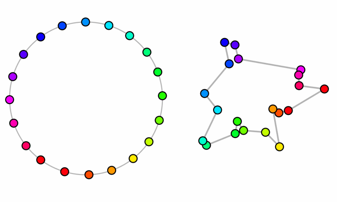
Ideally, only a strict minimum set of inductive biases are embedded within the solver and the rest should be handled by the neural network. We argue that a solver should embed the cyclic nature of the TSP directly into its output space. By mapping the N cities onto a unit circle, we represent the tour as a sequences of angles (a_i)_1^N. The tour is recovered simply by sorting the cities by their angular position. This approach offers three distinct advantages:
- Direct Decoding: Our representation is always valid. Any set of N distinct angles defines a valid Hamiltonian cycle, removing the need for complex post-processing.
- Generative Flexibility: Because the representation is continuous, we can leverage Flow Matching to treat solving as an ODE-based refinement process. We design a specific loss that takes into account the circular invariances of our solution representation.
- Variable NFEs: By using an ODE solver, we decouple the solving effort from the number of cities. We can refine a solution using 10, 100 or 1000 Number of Function Evaluations (NFEs), allowing for a dynamic trade-off between speed and optimality gap.
Solution Representation
A TSP instance is defined by a set of N cities with coordinates X = \{x_i\}_1^N \in \mathbb{R}^{N \times 2}. The objective is to find a permutation p of the indices \{1, \dots, N\} that minimizes the Hamiltonian cycle cost:
\sum_{i = 1}^{N - 1} ||x_{p_i} - x_{p_{i+1}}||_2 + ||x_{p_N} - x_{p_1}||_2.
We consider the cyclic nature of the solution and place the cities onto the unit circle. Each city i is assigned to an angular coordinate a_i \in [0, 2\pi). The set of all angles a = (a_1, \dots, a_N) implicitly defines a tour: the sequence is recovered by sorting cities according to their angular positions.
To train our models, we must map an optimal permutation p^* to a target angular configuration. We distribute the cities in the optimal tour uniformly along the circle:
a_{p_i^*} = a_i^* = \frac{2 \pi i}{N} \quad \forall i \in \{1, \dots, N\}.
Circular Flow Matching
We cast the generation of the tour as a flow matching problem. We assume some familiarity with the method, a thorough introduction to general flow matching can be found in Holderrieth et al., 2026. The goal is to learn a time-dependent vector field f_\theta that transports a distribution of random initial angles toward the target optimal configuration. At t = 0, the angles are randomly initialized following the uniform distribution a(0) \sim U[0, 2\pi]^N. The target state a(1) = a^* are the angles corresponding to the optimal tour. Using the optimal transport formulation, the flow is defined as the shortest path between a(0) and a(1), thus the neural network is involved in the Ordinary Differential Equation (ODE)
\frac{da(t)}{dt} = f_\theta(a(t), t, X).
The optimal solution on the circle is invariant to global rotations, so it would be inefficient to ask for the model to predict a particular angle position. Instead, we characterize the generated solution: we compute a one-step estimate of the solution, \hat{a}, and compare the pairwise angular distances between \hat{a} and that of the optimal tour a^*. Our loss is as follows:
\mathcal{L_{\text{cycle}}}(\theta) = || D(\hat{a}) - D(a^*) ||_2^2, \quad \hat{a} = a(t) + (1 - t) f_\theta(a(t), t, X)
where D \in \mathbb{R}^{N \times N \times 2} is the matrix of pairwise signed distances:
D(\hat{a})_{i, j} = \begin{pmatrix} \cos \hat{a}_i - \cos \hat{a}_j \\ \sin \hat{a}_i - \sin \hat{a}_j \end{pmatrix}.
This loss is rotationally invariant.
Neural Network Architecture
We treat the TSP instance as a complete graph where each city i is represented as a token of a Transformer neural network. Each token is initialized by projecting the concatenation of the city's coordinates x_i and the current flow timestep t into the dimension of the model d_\text{model}.
To properly encode the current state of the solution, we design the model to be invariant to global rotations of the circle. To do so, our model must perceive the angles relatively to each other: we adapt Rotary Positional Embeddings (RoPE, Su et al., 2021) which encodes the relative distance between discrete positions m and n. We instead define the position of a token as its continuous angle a_i \in [0, 2\pi). The transformation of the query q and key k vectors is defined as:
\text{RoPE}(q, a) = \begin{pmatrix} \cos a \theta_1 & -\sin a \theta_1 & 0 & 0 & \dots \\ \sin a \theta_1 & \cos a \theta_1 & 0 & 0 & \dots \\ 0 & 0 & \cos a \theta_2 & -\sin a \theta_2 & \dots \\ 0 & 0 & \sin a \theta_2 & \cos a \theta_2 & \dots \\ \vdots & \vdots & \vdots & \vdots & \ddots \end{pmatrix} \begin{pmatrix} q_1 \\ q_2 \\ q_3 \\ q_4 \\ \vdots \end{pmatrix} = \hat{q}
The resulting attention score is proportional to the cosine of the angular difference:
\hat{q}_m \hat{k}_n^T \propto \text{cos}((a_m - a_n) \theta).
For the model to be invariant, an angular shift of 2\pi must leave the representation unchanged:
\text{cos}\left( (a_m - a_n + 2k\pi) \theta \right) = \text{cos}\left( (a_m - a_n) \theta \right), \quad \forall k \in \mathbb{Z}
This condition is satisfied if and only if the frequency basis \theta consists of integers. In standard RoPE, these frequencies are typically real-valued and follow an exponential decay. To satisfy the circular constraint while maintaining a multi-scale representation of the circle, we introduce CircularRoPE. We define a set of integer frequencies (\theta_j)_{j = 1}^{d / 2} as follows:
\theta_j = \left\lfloor K_{ \text{max} }^{ \frac{2 j}{d} } \right\rceil,
where d is the head dimension and K_\text{max} controls the highest frequency (we use K_\text{max} = 5). By rounding the frequencies to the nearest integer, we ensure that every head in the attention mechanism respects the periodic topology of the solution. This makes the entire architecture naturally invariant to global rotations of the current input solution.
Timestep Sampling and the Refinement Bias
In standard flow matching, the timestep t is typically sampled from a uniform distribution, t \sim \mathcal{U}[0, 1], ensuring that the model learns to estimate the vector field equally well at all stages of the trajectory. However, we observed that for the TSP the task difficulty is non-uniformly distributed across time.
At the beginning of the flow t \approx 0, the cities' angles are near-random making the flow prediction much harder. When trained with uniform sampling, the model tends to exhaust its capacity trying to minimize error in these early stages, at the expense of precision in the final refinement phase (t \approx 1).
To prioritize those refinement steps, we sample timesteps from a Beta distribution t \sim \text{Beta}(\alpha, \beta). By setting \alpha = 5 and \beta = 1 the sampling density is heavily biased toward t = 1, which forces the neural network to focus on the end of the solving process.
Experiments
All instances are randomly generated by sampling points uniformly on the
unit square and using Concorde (Applegate et al., 2006) to generate optimal solutions. Training datasets contains 1M random
instances. Performance is measured with the optimality gap
\text{gap}(\%) = 100 * \frac{\text{cost}_{\text{pred}}}{\text{cost}_{\text{opt}}}.
We report the total inference time in minutes for the entire 128 test instances of each category.
Initial experiment. We first train three models for three different TSP sizes: 20, 50 and 100. Models are trained for 100k iterations with a batch size of 256. Models are similar to BQ-NCO and have 3M parameters. Once trained, we use the Euler ODE solver and specify the number of solver steps.
| Instance | 1 step | 10 steps | 100 steps | 1000 steps | ||||
|---|---|---|---|---|---|---|---|---|
| Gap | Time | Gap | Time | Gap | Time | Gap | Time | |
| TSP-20 | 20.92 | 0.9m | 0.35 | 0.9m | 0.26 | 1.0m | 0.26 | 1.6m |
| TSP-50 | 74.21 | 1.2m | 3.77 | 1.2m | 2.97 | 1.4m | 2.89 | 1.8m |
| TSP-100 | 167.21 | 1.1m | 7.73 | 1.2m | 5.05 | 1.2m | 4.83 | 1.8m |
Flow matching naturally handle the tradeoff between computation time and solution quality. We can see for example that TSP-50 can reach a pretty good solution in only 10 ODE steps (10 NFEs), but that going up to 1000 steps further improve the solution.
Problem-size Generalization. In a second example, we train a 25M parameters neural solver on training instances of sizes between 128 and 256. The variable training TSP sizes enhance the solver ability to generalize to larger instances.
| Model | TSP-100 | TSP-250 | TSP-500 | |||
|---|---|---|---|---|---|---|
| Gap | Time | Gap | Time | Gap | Time | |
| Ours (100 steps) | 5.67 | 1.4m | 11.01 | 1.8m | 29.00 | 1.3m |
| Ours (1000 steps) | 5.28 | 2.4m | 9.76 | 3.1m | 27.95 | 3.6m |
| BQ-NCO | 0.31 | 0.6m | 0.67 | 1.5m | 1.17 | 3.8m |
| INViT-3V | 4.95 | 1.0m | 5.92 | 2.8m | 6.30 | 5.9m |
We report the performance of our neural solver when using 100 and 1000 ODE solver steps. We compare against two well-known baselines, BQ-NCO (Drakulic et al., 2023) and INViT (Fang et al., 2024). As expected, our solutions generated with only 100 NFEs are much faster to produce, but sadly even with 1000 NFEs our model is not competitive.
Ablations. We now evaluate the pertinence of CircularRoPE and our flow matching loss. For CircularRoPE, we compare the TSP-100 model against a baseline that does not round the basis \theta (RoPE) and a third baseline that simply initialize the transformer tokens with their corresponding angles (Input Features).
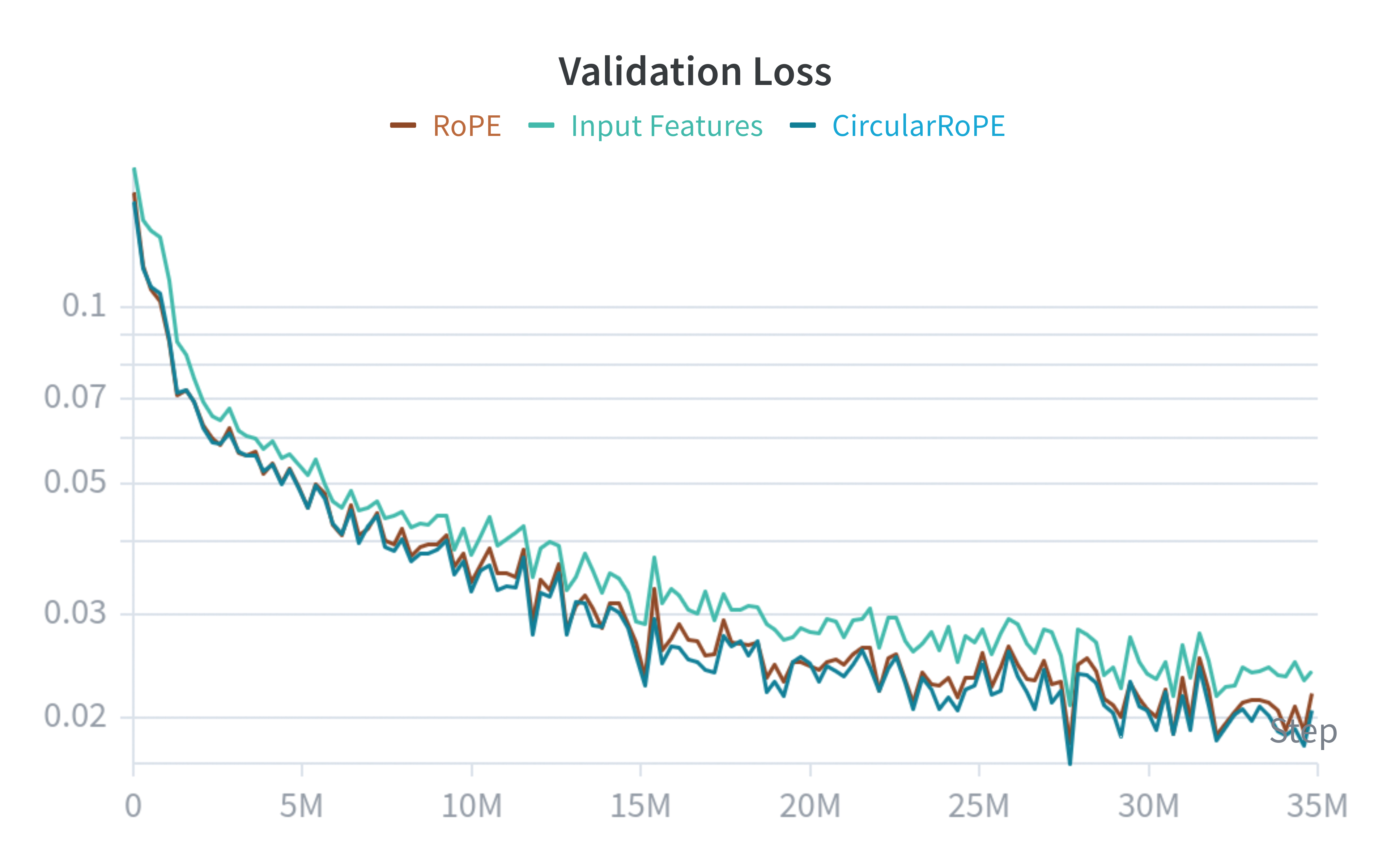
We can see that CircularRoPE and RoPE are slightly faster to train compared to the third baseline, but all of them plateau at the same spot. It appears that CircularRoPE do not make much of a difference against the classical RoPE, probably because RoPE is already almost circular invariant (up to some rounding error).
We now evaluate our circular invariant flow loss. We compare against the usual flow matching loss: \mathcal{L}(\theta) = || f_\theta(a(t), t, X) - \text{flow}(a(0), a(1)) ||_2. We also validate the beta distribution sampling of our timesteps by replacing it by the usual uniform sampling: t \sim U[0, 1].
| Model | TSP-100 |
|---|---|
| Baseline | 8.35 |
| + \mathcal{L}_{\text{cycle}}(\theta) | 7.42 |
| + t \sim \text{Beta}(5, 1) | 5.05 |
The original flow loss imposes a non-necessary constraint where the model has to predict the absolute angular positions. Adding our specific loss improves from 8.35\% to 7.42\%. Finally, biasing the training sampling of t to follow the \text{Beta}(5, 1) distribution forces the solver to focus on later stages of the solving process and further boost performances to 5.05\%.
Analysis
We experimentally saw a performance ceiling on TSP-100 instances, even when training larger models. This suggests that there is a fundamental issue with our approach.
We hypothesize that OT flow matching suffers from a high-cost correction problem: early trajectory mistakes are difficult to rectify because the transport cost of moving those points to the correct region of the circle is too high to be well-represented in our optimal transport training data. This may explain why we observe points that are locally well-ordered but trapped in the wrong global region of the circle.
Another possibility is that continuous models are prone to mode-averaging. Unlike discrete models that can output a multimodal probability distribution over cities, our models must predict a single scalar position. For example, if a model is uncertain between two valid positions, the MSE loss encourages it to predict the mean, which would result in a degenerate solution. In contrast, a discrete model would maintain both modes, allowing for a valid choice during decoding. A potential solution could be to project the tour into a latent space using a VAE (Kingma et al., 2013) and perform flow matching there where it is easier to express competing possibilities in a higher-dimensional manifold.
Finally, improvements like our biased sampling and the invariant flow loss helped to go from 8.35% to 5.05%, similar ideas might be necessary to make it competitive with other state-of-the-art methods.
We hope for this post to inspire other researchers to create NCO solvers with the least inductive biases as possible.
If you wish to cite this work, please use the following:
@misc{pereira_2026_20037323,
  author       = {Pereira, Pierre},
  title        = {Encoding the TSP Solution on a Circle},
  month        = mar,
  year         = 2026,
  publisher    = {Pierre Pereira},
  doi          = {10.5281/zenodo.20037323},
  url          = {https://doi.org/10.5281/zenodo.20037323},
  howpublished = {\url{https://pierrot-lc.dev/posts/circular-tsp/}},
}
References
-
BQ-NCO: Bisimulation Quotienting for Efficient Neural
Combinatorial Optimization
Drakulic, D., Michel, S., Mai, F., Sors, A., Andreoli, J., 2023, Advances in Neural Information Processing Systems, Curran Associates, Inc. -
RoFormer: Enhanced Transformer with Rotary Position
Embedding
Su, J., Lu, Y., Pan, S., Murtadha, A., Wen, B., Liu, Y., 2021, arXiv, DOI: 10.48550/ARXIV.2104.09864 -
INViT: a generalizable routing problem solver with invariant
nested view transformer
Fang, H., Song, Z., Weng, P., Ban, Y., 2024, Proceedings of the 41st International Conference on Machine Learning, JMLR.org -
DIFUSCO: graph-based diffusion solvers for combinatorial
optimization
Sun, Z., Yang, Y., 2023, Proceedings of the 37th International Conference on Neural Information Processing Systems, Curran Associates Inc. -
Concorde TSP Solver
Applegate, D., Bixby, R., Chvatal, V., Cook, W., 2006 -
Introduction to Flow Matching and Diffusion Models
Holderrieth, P., Erives, E., 2026 -
Auto-Encoding Variational Bayes
Kingma, D., Welling, M., 2013, arXiv, DOI: 10.48550/ARXIV.1312.6114